Graphical User Interface
Spectro package contains sviewer - the graphical user interface for the interactive spectral data analysis. It is located in the separate folder sviewer.
Run
sviewer GUI can be run using path/to/spectro/sviewer/__main__.py, for example:
$ path/to/python.exe path/to/spectro/sviewer/__main__.py
Alternatively, one can use convenient IDE to run the __main__.py, for example PyCharms, Spider, MScode, etc.
Main window
The main window of sviewer is typically looks like
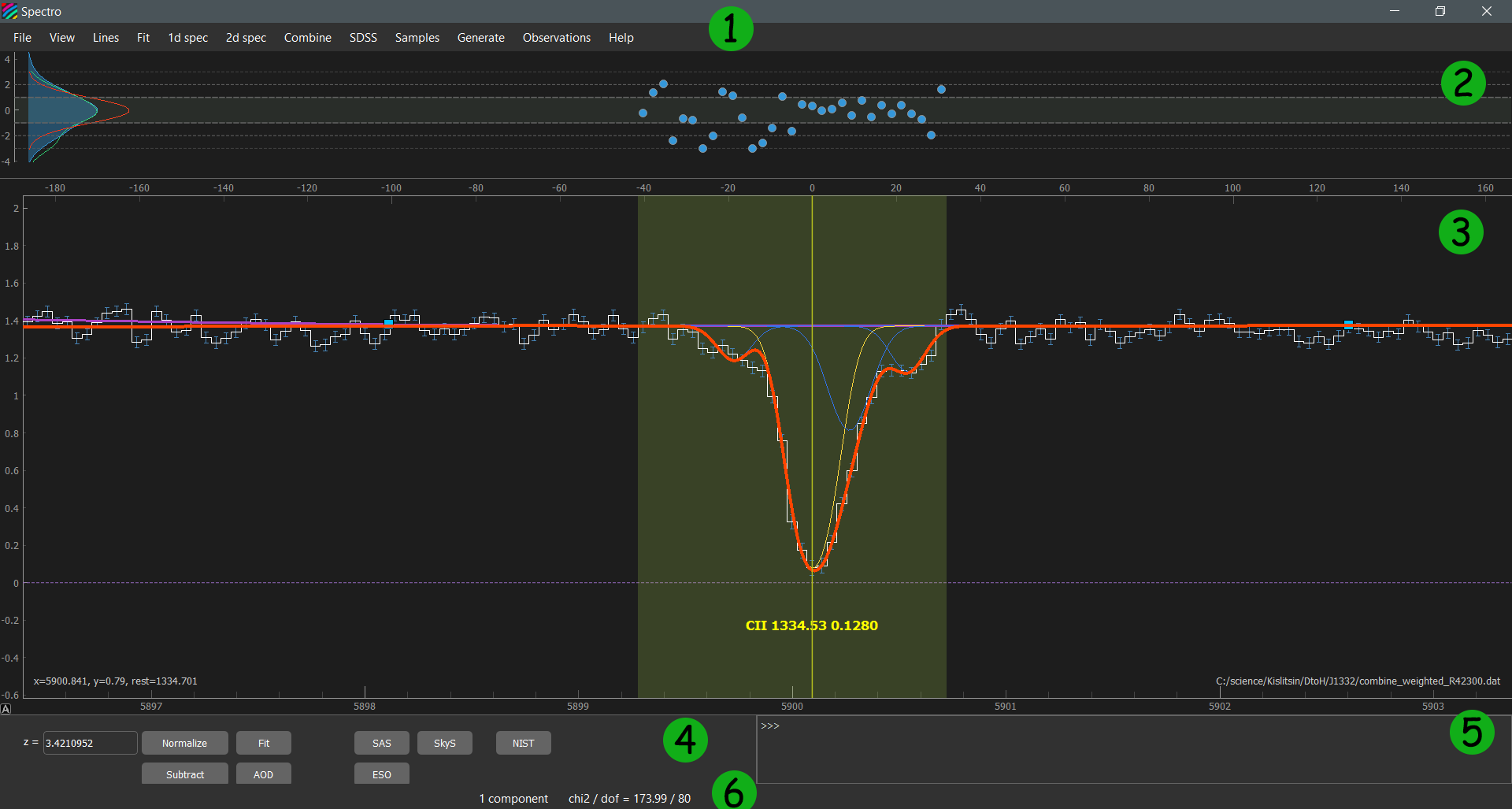
where numbers highlight the following parts of GUI:
Residuals panel
It shows the residuals between spectrum and the fit model. It has shared x-axis with the Spectrum panel. Residuals panel can be shown/hide by pressing F4 or view/Residuals in the Main Menu. The blue area and green line in the left of this panel show the kde of the residual distribution, that is calculated using pixels from the whole spectrum and from the view window only, respectively. The red line shows the gaussian function with unit dispersion, that should be approaching in case of good fit. Note: that consistency between blue and red lines are not necessary means reliable fit, since you also need to control the structure in residuals.
Spectrum panel
The main interactive window to work with the spectra. It shows the spectrum and the fit model and different graphical objects suitable for the spectral analysis. It is build on the base of PlotWidget class from the pyqtgraph package. The interaction process is quite essential, but the description of the main features of the interaction module can be find in the pyqtgraph manual, for example mouse interaction.
Control panel
This panel contains some useful buttons for the spectral analysis, including:
Redshift line edit field: input the redshift for the line markers shown in Spectrum panel. The redshift also can be changed either by moving line markers
SHIFT``+ drag or by using ``LEFTandRIGHTkeys on the keyboard (and also withSHIFT+LEFTandSHIFT+RIGHT).Normalize: switch between normalized and raw views (where continuum is explicitly shown), i.e. NORMALIZED = I/I_0
Subtract: switch between subtracted and raw views, i.e. SUBTRACTED = I-I_0
AOD: switch between apparent optical depth and raw views, i.e. AOD = np.ln(-I/I_0)
Fit: start the fit using LM minimization routine.
SAS: open spectrum in SDSS science archive server (only for SDSS spectra)
SkyS: open spectrum in SDSS sky server (only for SDSS spectra)
ESO: open spectrum in ESO data archive (not available yet)
NIST: show the list of the possible lines available in the NIST database which can be located within the
Regionobject within Spectrum panel taking into account specified redshift.
Console
It allows to input commands mostly concerned with GUI management. For the detailed descriptions see Console.
Status bar
Status bar shows some messages and indicate some useful numbers that are can be instructive during the fitting process, e.g. the number of the current fit component, chi^2/dof, etc